Week 3: Introduction to Unix/Linux and the Server; Assembly with IDBA-UD
Rika Anderson, Carleton College, Dec 23, 2017
Connecting to Liverpool
1. About Liverpool
We are going to do most of our computational work on a remote server (or computer) called Liverpool, which is a Linux virtual machine set up by Carleton ITS for our course. Liverpool basically lives in a computer somewhere in the CMC. You’ll be accessing it from the lab computers, but you could also access it from your own computer at home. First, you have to learn how to access Liverpool.
Boot as a Mac user on the lab computer.
2. Opening Terminal
Find and open the Terminal application (it should be in “Applications” in the folder called “Utilities”).
The terminal is the interface you will use to log in to the remote server for the rest of the course. It is also the interface we will be using to run almost all of the bioinformatics software we will be learning in this course. You can navigate through files on the server or on your computer, copy, move, and create files, and run programs using the Unix commands we learned earlier this week.
3. ssh
We will use something called ssh, or a secure socket shell, to remotely connect to another computer (in this case it will our class server, liverpool). Type the following:
ssh [username]@liverpool.its.carleton.edu
4. ssh (cont.)
You should see something like this: [your username]@liverpool.its.carleton.edu's password:
Type in your Carleton password. NOTE!! You will not see the cursor moving when you type your password. Never fear, it is still registering what you type. Be sure to use the correct capitalization and be wary of typos.
5. pwd
Whenever you ssh in to liverpool, you end up in your own home directory. Each of you has your own home directory on liverpool. To see where you are, print your current working directory.
# How to print your working directory (find out where you are in the system)
pwd
6. Your path
You should see something like this: /Accounts/[your username]
This tells you what your current location is within liverpool, also known as your path. But before we actually run any processes, we need to learn a few important things about using a remote shared server.
Important things to know about when using a remote shared server
7. top
One of the most important things to learn when using a remote shared server is how to use proper server etiquette. You don’t want to be a computer hog and take up all of the available processing power. Nobody earns friends that way. Similarly, if it looks like someone else is running a computationally intensive process, you might want to wait until theirs is done before starting your own, because running two intensive processes at the same time might slow you both down.
To see what other processes are being run by other users of the same server, type: top
You should see something like this:
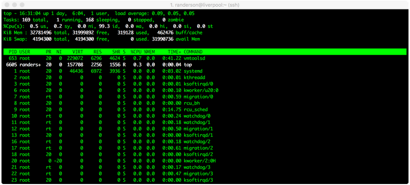
Here, we can see that randerson is the only user on liverpool, I am using a process called top, and it’s taking up 0.3% of one central processing unit (CPU), and zero memory. Not much is going on in this case. (All the other things listed under ‘root’ are processes that the computer is running in the background.) If someone’s process says 100.0 or 98.00 under %CPU, it means they’re using almost one entire CPU. Liverpool has 10 CPUs and 32 gigabytes of RAM total. Therefore, we can use up to 10 CPUs. If we try to overload the computer, it means that everyone else’s processes will have to be shared among the available CPUs, which will slow everyone down. If it looks like all 10 CPUs are already being used at a particular time, you might want to wait until later to run your own process.
To quit out of top, type: q
8. screen
Sometimes we will run processes that are so computationally demanding that they will run for several hours or overnight. Some processes can sometimes take several days, or even weeks. In order to run these processes, you want to be able to close out your session on the remote server without terminating your process. To do that, you use screen. Type: screen
Your terminal will open a clean window. You are now in a screen session. Any processes you start while you are in a screen session will continue running even after you log off of the remote server.
Let’s say you’ve typed the commands for a process, and now you’re ready to exit your screen session to let it run while you do other things. To leave the screen session, type: Control+A d
This will “detach” you from the screen session and allow you to do other things. Your screen session is still running in the background.
To resume your screen session to check on things, type: screen -r. (Now you’ve re-entered your screen session.)
To kill your screen session (this is important to tidy up and keep things neat when your process is finished!) type: Control+A k.
- The computer will say:
Really kill this window [y/n]. You type:y. - If this doesn’t work, you can also type
exitto terminate the screen session.
Creating an assembly and evaluating it (toy dataset)
9. mkdir
Let’s say we’ve gone out in to the field and taken our samples, we’ve extracted the DNA, and we’ve sent them to a sequencer. Then we get back the raw sequencing reads. One of the first things we have to do is assemble them. To do that, we’re going to use a software package called IDBA-UD. Bioinformaticians love to debate about which assembler is best, but ultimately it usually depends on the nature of your own dataset. If you find yourself with data like this someday and you want to know which assembler to use, my advice is to try a bunch of them and then compare the results using something like Quast, which we’ll test below. For now, we’re going to use IDBA-UD, which I’ve found to be a good general-purpose assembler.
Make a new directory in your home folder:
mkdir toy_dataset_directory
11. Copy toy dataset
Copy the toy dataset into your assembly directory. Don’t forget the period at the end! This means you are copying into the directory you are currently in.
cp /usr/local/data/toy_datasets/toy_dataset_reads.fasta .
12. Run idba-ud on toy dataset
Run idba-ud on the toy dataset. Here is what these commands mean:
- Invoke the program
idba-ud - The
-rgives it the “path” (directions) to the reads for your toy dataset.../means it is in the directory outside of the one you’re in. - The
-oflag tells the program that you want the output directory to be called “toy_assembly”
idba_ud -r toy_dataset_reads.fasta -o toy_assembly
13. cd to output directory
When that’s done running, go into your new output directory and take a look at what’s inside:
cd toy_assembly
ls
14. The output files
You should see several files, including these:
contig.fa
contig-20.fa
contig-40.fa
contig-60.fa
contig-80.fa
contig-100.fa
scaffold.fa
You may recall that De Bruijn graph assembly works by searching reads for overlapping words, or “kmers.” IDBA-UD starts by searching for small kmers to assemble reads into longer contigs. Then it uses those constructed contigs for a new round of assembly with longer kmers. Then it does the same with even longer kmers. It iterates through kmers of length 20, 40, 60, 80, and 100. You should get longer and longer contigs each time. Each “contig-” file gives the results of each iteration for a different kmer size. The “scaffolds.fa” file provides the final scaffolded assembly, which pulls contigs together using the paired-end data.
15. Examine output
Let’s examine the assembly output files. First, take a look at your final scaffold output:
less scaffold.fa
16. Fasta file
You should see a fasta file with some very long sequences in it. When you’re done looking at it, type: q.
17. Evaluate assembly quality
Now we’re going to evaluate the quality of our assembly. One measure of assembly quality is N50, which is the contig length for which the collection of all contigs of that length or longer contains at least 50% of the sum of the lengths of all contigs. We could theoretically calculate the N50 by hand, but often times you’ll get many, many contigs and it’s very tedious to do by hand. So we will use an assembly evaluator called Quast. Run it on your toy dataset. (If you’ve been copying and pasting, it may not work here; you may have to type it in.) Here is what the commands mean:
- Invoke the program
quast.py - We tell it to run the program on all of the output files of your toy assembly. Every fasta file that we list after
quast.pywill be included in the analysis. - The
-oflag will create an output directory that we will calltoy_assembly_quast_evaluation
quast.py contig-20.fa contig-40.fa contig-60.fa contig-80.fa contig-100.fa scaffold.fa –o toy_assembly_quast_evaluation
18. View output with x2go
Quast gives you some nice visual outputs that are easiest to see if you log in to x2go. More detailed instructions are here:
https://wiki.carleton.edu/display/carl/How+to+Install+and+Configure+x2go+client
- Find x2go on your lab computer and open it.
- Click “New session” in the top left of the screen (it’s an icon with a piece of paper with a yellow star on it.)
- Enter “liverpool.its.carleton.edu” in the Host box. Choose the SSH port to be 22. The session type should be XFCE. You can set the session name to “Liverpool” or whatever you like. Click OK.
- Click on your newly created session, which should appear on the right side of the window.
- Log in with your Carleton account name and password.
- Navigate to the directory called “toy_assembly_quast_evaluation.”
- Double-clock on the file called “report.html” and take a look. It reports the number of contigs, the contig lengths, the N50, and other statistics for each of the assembly files you entered. The graph at the bottom shows the cumulative length of your assembly (y-axis) as you add up each contig in your assembly (x-axis). Many of your lab questions for this week are based on the quast assembly report.
- When you are done with x2go, be sure to click on “Log Out” when you log out!
19. Bookkeeping
For the sake of future bookkeeping, you’ll need to modify your scaffold assembly file so that another software program we will use in the future (called anvi’o) is happy. (Spaces and other weird characters are so tricky sometimes.) This will be very important for your project datasets as well. Do this while you are inside the directory with your assembly files:
anvi-script-reformat-fasta scaffold.fa -o toy_dataset_assembled.fa -l 0 --simplify-names
Create and evaluate assembly (project dataset)
20. screen
You’re now going to run an assembly on your project dataset. Since this will take about 10-20 minutes, I recommend running this on screen. Type:
screen
21. cd
Make a new directory in your home folder called “project_directory,” and then change directory into your newly created directory:
cd ~
mkdir project_directory
cd project_directory
22. Copy project dataset
Next, copy your project dataset in to that directory. Your assigned project dataset is listed in an Excel file that is on the Moodle.
For example, if you have dataset ERR590988 from the Arabian Sea, you would do this:
cp /usr/local/data/Tara_datasets/Arabian_Sea/ERR598966_sample.fasta .
23. Start assembly
Next, start your assembly. Substitute the name of your own sample dataset for the dataset shown here.
idba_ud -r ERR598966_sample.fasta -o ERR598966_assembly
24. Detach from screen
This is likely to take a little while. After you’ve started the process, detach from screen:
Ctrl+A d
To check on the progress of your assemblies, you can either use top to see if your assembly is still running, or you can re-attach to your screen using the instructions above.
When IDBA-UD finishes, it will say:
invalid insert distance
Segmentation fault
This is because we gave IDBA-UD single-end reads instead of paired-end reads. Never fear! Despite appearances, your assembly actually did finish. However, the use of single-end reads instead of paired-end reads means that your assemblies will NOT have scaffolds, because we couldn’t take advantage of the paired-end data to make scaffolds. So, your final assembly is just the final contig file from the longest kmer, called contig-100.fa.
25. Rename assembly
When your project assembly is done, change the name of your final assembly from contig-100.fa to a name that starts with your dataset number, followed by _assembly.fasta. For example, you might call it something like ERR598966_assembly.fasta.
This way we will have standardized names and save ourselves future heartache. (For a reminder on how to change file names, see your Unix cheat sheet.)
26. Run anvi
Run anvi-script-reformat-fasta on your completed project assemblies (see step 19 for instructions).
27. Exit
When you are all done with your work on the server, you can log off the server by typing:
exit
NOTE!!! If you type this while you are still in screen it will kill your screen session! Be sure to detach from screen first if you want to let your process keep running after you log off the server.
These assemblies will likely take some time. Take advantage of your time in lab to discuss the following questions with your colleagues. I encourage collaboration and sharing of ideas, but I expect each of you to submit your own assignment, which should reflect your own ideas and understanding of the responses.
Questions to answer for this week
28. Questions
Consider and answer the following questions and submit a Word document with your responses on the Moodle by lab time next week.
Check for understanding:
Q1. (a-d) About your toy dataset assembly:
- How many reads did you start with in the raw data file for your toy dataset, prior to assembly? (Hint: refer to the Unix tutorial you did, and use grep to search for the ‘>’ symbol that denotes each new sequence. The > symbol also means something in Unix, so be sure to use quotes around it!)
- Examine the Quast output. Describe and explain the pattern you observe in terms of N50 as the kmer size increases (from ‘contig-20.fa’ all the way to ‘contig-100.fa’).
- Examine the Quast output. How does the N50 of your scaffold file compare to your contig-100 file? Explain why.
- Examine the Quast output. Which assembly output file had the most contigs? The fewest? Explain why.
Critical thinking:
Q2. Let’s say that in preparing your samples for sequencing, you sheared your DNA to create an insert size (DNA sequence length) of 200 bp, and you sequenced them on an Illumina machine with 200 bp reads. How would you expect your scaffolds file to differ from your contig-100 file? What if you had instead selected an insert size of 500 bp? Explain your reasoning.
Q3. Describe why a CRISPR array (see here for a reminder of what that looks like) might present a problem for assembly and what strategies you might use to overcome this problem.
Q4. If you were testing different types of assembly software on a metagenome with high coverage, and one used k-mers of length 40 and the other used k-mers of length 20, how would you expect the N50 and total assembly length to differ and why? In contrast, if you were testing them on a metagenome with low coverage, would you expect the same results?
Q5. Last week, we sampled water bodies within the Cannon River watershed. In the winter, you tend to get a very diverse microbial community, with lots of single nucleotide variants differentiating the microbes. In contrast, in spring or fall after a heavy rainfall, you might expect that nutrient runoff would go into the lakes, leading to a bloom of one specific type of microbe with very few single nucleotide variants, creating a less diverse microbial community. How might you expect your assembly N50 to differ between the winter and spring/fall communities? (You should include a discussion of coverage and de Bruijn graph construction in your answer.)